Take-Home Exercise 01

1. Task Background

City of Engagement, with a total population of 50,000, is a small city located at Country of Nowhere. The city serves as a service centre of an agriculture region surrounding the city. The main agriculture of the region is fruit farms and vineyards. The local council of the city is in the process of preparing the Local Plan 2023. A sample survey of 1000 representative residents had been conducted to collect data related to their household demographic and spending patterns, among other things. The city aims to use the data to assist with their major community revitalization efforts, including how to allocate a very large city renewal grant they have recently received.

2. Task

• Reveal demographic and financial characteristics of the city of Engagement, using appropriate static and interactive statistical graphics methods.
  
• Provide user-friendly and interactive solutions for data exploration using ggplot2.

3. Data

Dataset 1 - Participants.csv

Contains information about the residents of City of Engagement that have agreed to participate in this study.

Participants.csv Dataset

Column Name	Data Type	Description
participantId	integer	unique ID assigned to each participant
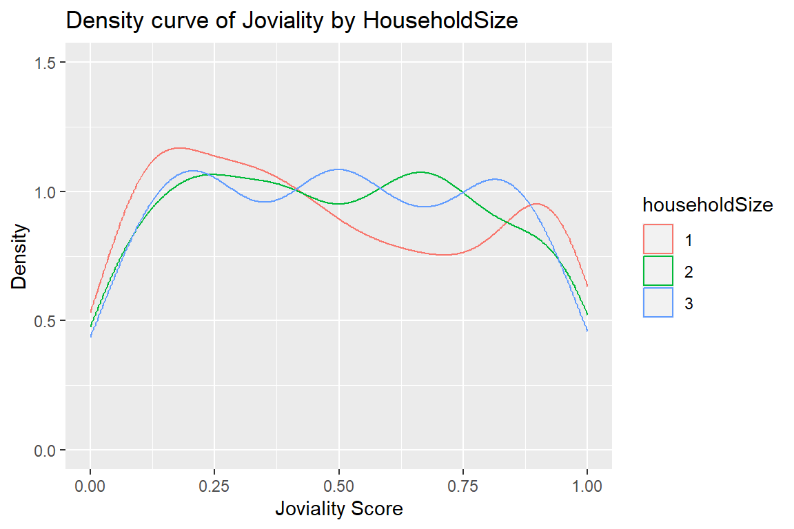
householdSize	integer	the number of people in the participant’s household
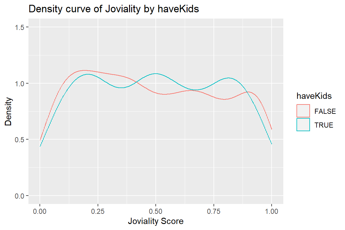
haveKids	boolean	whether there are children living in the participant’s household
age	integer	participant’s age (in years) at the start of the study
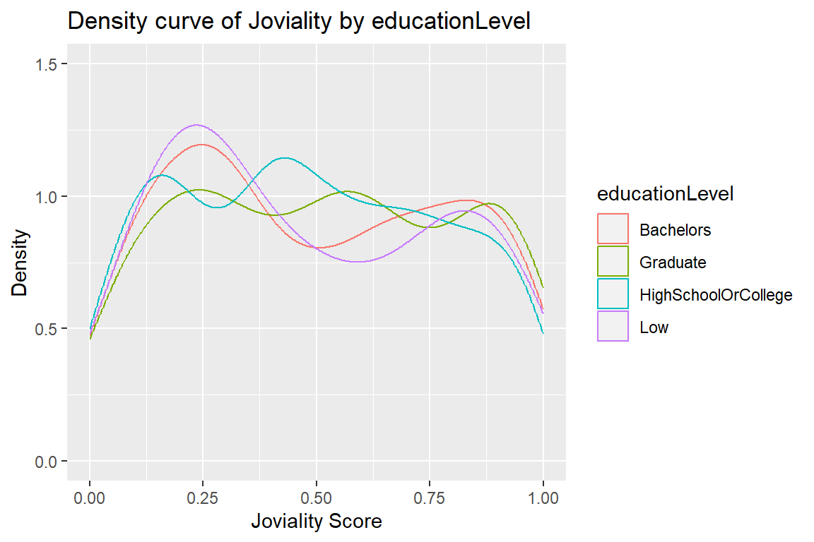
educationLevel	string factor	the participant’s education level, one of: {“Low”, “HighSchoolOrCollege”, “Bachelors”, “Graduate”}
interestGroup	char	a char representing the participant’s stated primary interest group, one of {“A”, “B”, “C”, “D”, “E”, “F”, “G”, “H”, “I”, “J”}. Note: specific topics of interest have been redacted to avoid bias.
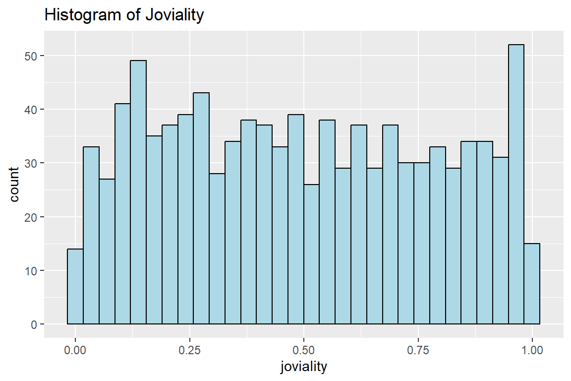
joviality	float	a value ranging from [0,1] indicating the participant’s overall happiness level at the start of the study.

Dataset 2 - FinancialJournal.csv

Contains information about financial transactions.

FinancialJournal.csv Dataset

Column Name	Data Type	Description
participantId	integer	unique ID corresponding to the participant affected
timestamp	datetime	the time when the check-in was logged
category	string factor	a string describing the expense category, one of {“Education”, “Food”, “Recreation”, “RentAdjustment”, “Shelter”, “Wage”}
amount	double	the amount of the transaction

4. Data Preparation

4.1 Install and launch R packages

The following packages will be used for this assignment.

pacman::p_load(tidyverse, ggrepel, patchwork, ggthemes, hrbrthemes, ggiraph, plotly, DT, readxl, gifski, gapminder, gganimate, webshot2, ggstatsplot, gt, dplyr, rstatix, ggpubr, ggdist, ggridges, colorspace, ggplot2, car) 

package 'ggiraph' successfully unpacked and MD5 sums checked

The downloaded binary packages are in
    C:\Users\User\AppData\Local\Temp\RtmpMXtkEF\downloaded_packages
package 'gifski' successfully unpacked and MD5 sums checked

The downloaded binary packages are in
    C:\Users\User\AppData\Local\Temp\RtmpMXtkEF\downloaded_packages
package 'gapminder' successfully unpacked and MD5 sums checked

The downloaded binary packages are in
    C:\Users\User\AppData\Local\Temp\RtmpMXtkEF\downloaded_packages
package 'gganimate' successfully unpacked and MD5 sums checked

The downloaded binary packages are in
    C:\Users\User\AppData\Local\Temp\RtmpMXtkEF\downloaded_packages
package 'distributional' successfully unpacked and MD5 sums checked
package 'ggdist' successfully unpacked and MD5 sums checked

The downloaded binary packages are in
    C:\Users\User\AppData\Local\Temp\RtmpMXtkEF\downloaded_packages
package 'ggridges' successfully unpacked and MD5 sums checked

The downloaded binary packages are in
    C:\Users\User\AppData\Local\Temp\RtmpMXtkEF\downloaded_packages

4.2 Loading datasets

participant <- read_csv("data/Participants.csv")
finances <- read_csv("data/FinancialJournal.csv")

4.3 Data Preparation

Participant

No duplicated rows found.

dim(participant)

[1] 1011    7

participant <- participant %>% distinct()
dim(participant)

[1] 1011    7

Finances

Removal of 1113 duplicated rows.

dim(finances)

[1] 1513636       4

finances <- finances %>% distinct()
dim(finances)

[1] 1512523       4

4.3.1 Merging Datasets

Merging datasets of Participant.csv and FinancialJournal.csv by the common column “participantId”.

Extract of Data Table

Code

joined_df <- merge(participant, finances, by.x = "participantId", 
             by.y = "participantId", all.x = TRUE, all.y = FALSE)
datatable(data=head(joined_df,200), filter = "top")

4.3.2 Participant Expenditures by Month & Year for Each Category

To show the total finances by participant, we will first extract the Year and Month using the “extract” function. Next we will use “pivot_longer” consolidate all the expenditures to “spending” and use “pivot_wider” to extract the expenditure for each category.

We will also add a sum of total monthly spent as a new column.

Extract of Data Table

Code

finances_aggregated<-finances %>% 
  mutate(
    Month_Year = format(as.Date(joined_df$timestamp), "%Y-%m")
  ) %>% 
  pivot_longer(-c(participantId, timestamp, category, Month_Year), values_to = "spending") %>%
  pivot_wider(names_from = category, values_from = spending, values_fn = list(spending=list)) %>% 
  unchop(everything()) %>% 
  mutate(
    Total_Monthly = select(., Wage:Recreation) %>% rowSums(na.rm = TRUE)
  )

finances_aggregated <- subset(finances_aggregated, select = -c(name, timestamp)) %>% 
  replace(is.na(.), 0)

datatable(data=head(finances_aggregated,200), filter = "top")

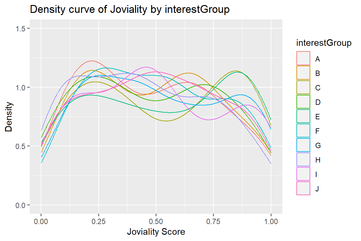
4.3.3 Participant Joviality by InterestGroups and haveKids

To deep dive in to possible analysis for demographic details for interest groups and those with/without kids, we will be deriving the count, mean, and standard deviation for these categories.

Data Table

Code

participantIG <- participant %>% 
  group_by(interestGroup,haveKids) %>% 
  dplyr::summarise(count = n(),
            Avg_Jov=mean(joviality,na.rm=TRUE),
            SD_Jov=sd(joviality,na.rm=TRUE))

datatable(data=participantIG, filter = "top")

4.4 Exploratory Data Analysis

4.4.1 Statistical overview

Participant.csv

We will change the class of “educationLevel”, “interestGroup”, and “householdSize” to factor in order to view their summary stats.

Code

participant$educationLevel <- as.factor(participant$educationLevel)
participant$interestGroup <- as.factor(participant$interestGroup)
participant$householdSize <- as.factor(participant$householdSize)

summary(participant)

 participantId    householdSize  haveKids            age       
 Min.   :   0.0   1:337         Mode :logical   Min.   :18.00  
 1st Qu.: 252.5   2:373         FALSE:710       1st Qu.:29.00  
 Median : 505.0   3:301         TRUE :301       Median :39.00  
 Mean   : 505.0                                 Mean   :39.07  
 3rd Qu.: 757.5                                 3rd Qu.:50.00  
 Max.   :1010.0                                 Max.   :60.00  
                                                               
             educationLevel interestGroup   joviality       
 Bachelors          :232    J      :116   Min.   :0.000204  
 Graduate           :170    H      :111   1st Qu.:0.240074  
 HighSchoolOrCollege:525    G      :108   Median :0.477539  
 Low                : 84    F      :106   Mean   :0.493794  
                            A      :102   3rd Qu.:0.746819  
                            C      :102   Max.   :0.999234  
                            (Other):366                     

In the correlation matrix below, we can observe that there are no strong correlation between the numeric variables.

Code

numvars <- c("age","joviality")
round(cor(participant[, numvars], use = "complete.obs"), 2)

            age joviality
age        1.00     -0.07
joviality -0.07      1.00

FinancialJournal.csv

We will change the class of “category” to factor in order to view the summary stats.

Code

finances$category <- as.factor(finances$category)
summary(finances)

 participantId      timestamp                                category     
 Min.   :   0.0   Min.   :2022-03-01 00:00:00.00   Education     :  3018  
 1st Qu.: 222.0   1st Qu.:2022-05-24 16:05:00.00   Food          :790051  
 Median : 464.0   Median :2022-08-25 16:20:00.00   Recreation    :296013  
 Mean   : 480.9   Mean   :2022-08-26 08:09:38.58   RentAdjustment:   131  
 3rd Qu.: 726.0   3rd Qu.:2022-11-27 08:05:00.00   Shelter       : 10651  
 Max.   :1010.0   Max.   :2023-02-28 23:55:00.00   Wage          :412659  
     amount         
 Min.   :-1562.726  
 1st Qu.:   -5.594  
 Median :   -4.000  
 Mean   :   20.423  
 3rd Qu.:   21.649  
 Max.   : 4096.526  

Finances_aggregated (Newly Formed)

We can see that expenditures categories are shelter, education, food, and recreation. Rent adjustment and wage are income earning categories.

Code

summary(finances_aggregated)

 participantId     Month_Year             Wage            Shelter         
 Min.   :   0.0   Length:1512027     Min.   :   0.00   Min.   :-1562.726  
 1st Qu.: 222.0   Class :character   1st Qu.:   0.00   1st Qu.:    0.000  
 Median : 464.0   Mode  :character   Median :   0.00   Median :    0.000  
 Mean   : 480.9                      Mean   :  30.16   Mean   :   -4.482  
 3rd Qu.: 726.0                      3rd Qu.:  21.65   3rd Qu.:    0.000  
 Max.   :1010.0                      Max.   :4096.53   Max.   :    0.000  
   Education        RentAdjustment           Food           Recreation    
 Min.   :-91.1435   Min.   :   0.0000   Min.   :-14.840   Min.   :-44.52  
 1st Qu.:  0.0000   1st Qu.:   0.0000   1st Qu.: -4.070   1st Qu.:  0.00  
 Median :  0.0000   Median :   0.0000   Median : -4.000   Median :  0.00  
 Mean   : -0.0926   Mean   :   0.0363   Mean   : -2.449   Mean   : -2.74  
 3rd Qu.:  0.0000   3rd Qu.:   0.0000   3rd Qu.:  0.000   3rd Qu.:  0.00  
 Max.   :  0.0000   Max.   :1506.1511   Max.   :  0.000   Max.   :  0.00  
 Total_Monthly      
 Min.   :-1590.397  
 1st Qu.:   -5.594  
 Median :   -4.000  
 Mean   :   20.429  
 3rd Qu.:   21.649  
 Max.   : 4096.526  

4.4.2 Visual overview

4.4.2.1 Participant.csv

The different tabs for Overview of Joviality with other variables

Overall

We can see that the jovality of the participants are generally equally distributed.

Code

ggplot(data=participant,aes(x=joviality)) +
  geom_histogram(fill='lightblue', color='black')+
  ggtitle("Histogram of Joviality")

HouseholdSize

For household size of 1, it’s noted that there is a lower proportion of participants who have the joviality scores between 0.5 to 0.8.

Code

ggplot(data=participant,aes(x=joviality, colour=householdSize)) +
  geom_density() +
  ggtitle("Density curve of Joviality by HouseholdSize") +
  scale_x_continuous(name="Joviality Score", limits=c(0,1)) +
  scale_y_continuous(name="Density", limits = c(0,1.5))

HaveKids

No notable proportional difference of joviality between those with kids and those without.

Code

ggplot(data=participant,aes(x=joviality, colour=haveKids)) +
  geom_density() +
  ggtitle("Density curve of Joviality by haveKids") +
  scale_x_continuous(name="Joviality Score", limits=c(0,1)) +
  scale_y_continuous(name="Density", limits = c(0,1.5))

Education Levels

We can see that there is a higher proportion of participants with “Low” and “Bachelors” education level that have the joviality scores around 0.25.

Code

ggplot(data=participant,aes(x=joviality, colour=educationLevel)) +
  geom_density() +
  ggtitle("Density curve of Joviality by educationLevel") +
  scale_x_continuous(name="Joviality Score", limits=c(0,1)) +
  scale_y_continuous(name="Density", limits = c(0,1.5))

Interest Groups

We note that those in interest groups C and D have a higher proportion of happier people with joviality scores more than 0.75.

Code

ggplot(data=participant,aes(x=joviality, colour=interestGroup)) +
  geom_density() +
  ggtitle("Density curve of Joviality by interestGroup") +
  scale_x_continuous(name="Joviality Score", limits=c(0,1)) +
  scale_y_continuous(name="Density", limits = c(0,1.5))

Normality Test

Code

qq <- ggplot(participant,
             aes(sample=joviality)) +
  stat_qq() +
  stat_qq_line()

sw_t <- participant %>% 
  shapiro_test(joviality) %>% 
  gt()

tmp <- tempfile(fileext = '.png')
gtsave(sw_t,tmp)

table_png <- png::readPNG(tmp, native = TRUE)

qq + table_png

Note

The p-value is less than 0.05, hence we reject the null hypothesis and conclude that the jovality scores does not follow a normal distribution.

4.4.4.2 FinancialJournal.csv

The different tabs for overview of finances by Expenditures and Earnings

Expenditures

Overview

Code

expenditurevar1 <- finances[which(finances$category %in% c("Education","Food","Recreation","Shelter")),]


p1 <- ggplot(data=expenditurevar1,aes(y=amount, x=category)) +
  geom_boxplot() +
  ggtitle("BoxPlot of Expenditures") 

p1 <- p1 + 
  scale_y_continuous(labels = scales::comma) +
  xlab("Categories") +
  ylab("Expenditures ($)")

ggplotly(p1)

Side-by-Side Comparison of Categories

we can see plot II, III, and IV are right skewed.

Code

expenditurevar2 <- finances[which(finances$category %in% c("Education")),]
expenditurevar3 <- finances[which(finances$category %in% c("Food")),]
expenditurevar4 <- finances[which(finances$category %in% c("Recreation")),]
expenditurevar5 <- finances[which(finances$category %in% c("Shelter")),]

p2 <- ggplot(data=expenditurevar2,aes(x=amount)) +
  geom_histogram(bins=20,color="grey25",fill="grey90") +
  ggtitle("Histogram: Education") 

p2 <- p2 + 
  scale_y_continuous(labels = scales::comma) +
  xlab("Expenditures") +
  ylab("Count")


p3 <- ggplot(data=expenditurevar3,aes(x=amount)) +
  geom_histogram(bins=20,color="grey25",fill="grey90") +
  ggtitle("Histogram: Food") 

p3 <- p3 + 
  scale_y_continuous(labels = scales::comma) +
  xlab("Expenditures") +
  ylab("Count")

p4 <- ggplot(data=expenditurevar4,aes(x=amount)) +
  geom_histogram(bins=20,color="grey25",fill="grey90") +
  ggtitle("Histogram: Recreation") 

p4 <- p4 +  
  scale_y_continuous(labels = scales::comma) +
  xlab("Expenditures") +
  ylab("Count")

p5 <- ggplot(data=expenditurevar5,aes(x=amount)) +
  geom_histogram(bins=20,color="grey25",fill="grey90") +
  ggtitle("Histogram: Shelter")

p5 <- p5 + 
  scale_y_continuous(labels = scales::comma) +
  xlab("Expenditures") +
  ylab("Count")

((p2 / p3 | p4 / p5) + plot_annotation(tag_levels='I'))

Earnings

Overview

Based on the overview plot, we can see that there are many extreme outliers for wages, hence we will remove the outliers for the histogram breakdown for wages. For the removal of outliers, we will take the max value as 3rd quantile + 1.5IQR (i.e. 137.2664857+(1.5*87.60608))

Code

earningvar <- finances[which(finances$category %in% c("Wage","RentAdjustment")),]
p3 <- ggplot(data=earningvar,aes(y=amount, x=category)) +
  geom_boxplot() +
  ggtitle("Boxplot of Earnings")

p3 <- p3 + 
  scale_y_continuous(labels = scales::comma) +
  xlab("Categories") +
  ylab("Earnings")

ggplotly(p3)

Side-by-Side Comparison of Categories

For plots I and II, we note that the earnings are left skewed, even after removal of outliers for wages.

Code

earningvarRA <- finances[which(finances$category %in% c("RentAdjustment")),]
p1 <- ggplot(data=earningvarRA,aes(x=amount)) +
  geom_histogram(bins=20,color="grey25",fill="grey90") +
  ggtitle("Histogram: Rent Adjustments")

p1 <- p1 + 
  scale_y_continuous(labels = scales::comma) +
  xlab("Earnings") +
  ylab("Count")

earningvarW <- finances[which(finances$category %in% c("Wage")),]
p2 <- ggplot(data=earningvarW,aes(x=amount)) +
  geom_histogram(bins=20,breaks=seq(0,268.6756),color="grey25",fill="grey90") +
  ggtitle("Histogram: Wage")

p2 <- p2 + 
  scale_y_continuous(labels = scales::comma) +
  xlab("Earnings") +
  ylab("Count")


((p1 | p2) + plot_annotation(tag_levels='I'))

5. Data Visualisation

5.1 Jovialty by Age Groups

As a data prep, we will extract age information from participant, and add in age ranges, as well as age groups for analysis.

Based on Singapore’s National Statistical Standards, we will group them in intervals of 5, with the last interval being 55-59 due to the distribution of age (i.e. max = 60).

National Statistical Standards

For age groups we will group them by age structure.

Age Structure

Age Group	Age Range
early_working_age	15-24
prime_working_age	25-54
mature_working_age	55-64

Code

participantage <- participant %>% 
  mutate(
    agerange = case_when(
      age <= 19 ~ "15-19",
      age <= 24 ~ "20-24",
      age <= 29 ~ "25-29",
      age <= 34 ~ "30-34",
      age <= 39 ~ "35-39",
      age <= 44 ~ "40-44",
      age <= 49 ~ "45-49",
      age <= 54 ~ "50-54",
      age <= 60 ~ "55-60"
    ),
    agegroup = case_when(
      age <= 24 ~ "early_working_age",
      age <= 54 ~ "prime_working_age",
      age <= 64 ~ "mature_working_age"
    )
  ) %>% 
  select(participantId,joviality,age,agerange,agegroup)

Observation 1 - Age Ranges that are Happier/Unhappier than General Population

Interactive Plot

We can see that those in the age ranges 15-19 and 25-29 are generally happier than the general population. On the other hand, we can also see that those in the age ranges 30-34 and 50-54 are generally unhappier than the general population.

Code

JAge <- plot_ly(
  data = participantage,
  y = ~joviality,
  x = ~agerange,
  type = "box",
  color = ~agegroup,
  boxmean=TRUE,
  notched=TRUE
) %>%
  layout(title = 'Boxplot of Joviality by Age Range',
         xaxis=list(title='Age Range'),
         yaxis=list(title='Joviality Score'),
         legend = list(title=list(text='Age Group'))) %>% 
  add_lines(
    y = mean(participantage$joviality),
    x = participantage$agerange,
    line = list(
      color = "purple"
    ),
    inherit = FALSE,
    showlegend = FALSE
  ) 
JAge

One-Way ANOVA Test

Earlier we determined that normality for joviality is not assumed. Hence we test the following hypothesis using non-parametric Kruskal Wallis Test.

H_0: There is no significant difference between the mean joviality of all the age groups.
H₁: There is significant difference between the mean joviality of all the age groups.

Code

kruskal.test(joviality ~ agerange, data = participantage)

    Kruskal-Wallis rank sum test

data:  joviality by agerange
Kruskal-Wallis chi-squared = 14.904, df = 8, p-value = 0.06104

Note

The p-value is not <0.05, hence we do not have enough evidence to conclude that there are significant difference between the age groups mean joviality at 95% confidence interval.

Observation 2 - No Notable Differences Between Working Age Groups

Interactive Plot

Code

JAgeWG <- plot_ly(
  data = participantage,
  y = ~joviality,
  x = ~agegroup,
  type = "box",
  color = ~agegroup,
  boxmean=TRUE,
  notched=TRUE
) %>%
  add_lines(
    y = mean(participantage$joviality),
    x = participantage$agegroup,
    line = list(
      color = "purple"
    ),
    inherit = FALSE,
    showlegend = FALSE
  ) 
JAgeWG

One-Way ANOVA Test

Earlier we determined that normality for joviality is not assumed. Hence we test the following hypothesis using non-parametric Kruskal Wallis Test.

H_0: There is no significant difference between the mean joviality of all the age groups.
H₁: There is significant difference between the mean joviality of all the age groups.

Code

kruskal.test(joviality ~ agegroup, data = participantage)

    Kruskal-Wallis rank sum test

data:  joviality by agegroup
Kruskal-Wallis chi-squared = 0.32849, df = 2, p-value = 0.8485

Note

The p-value is not <0.05, hence we do not have enough evidence to conclude that there are significant difference between the age groups mean joviality at 95% confidence interval.

5.2 Jovialty by Education Level with Financial Considerations

We can see that those who have Bachelors and Graduate education tend to have higher expenditures, followed by those who received High School/College and lastly those who have Low education levels.
We also see that with increase in expenditure, there is an exponential decline in joviality scores.

Plot

Plot Code

finances_aggregated<-joined_df %>% 
  mutate(
    Month_Year = format(as.Date(joined_df$timestamp), "%Y-%m")
  ) %>% 
  group_by(participantId,joviality,educationLevel) %>% 
  summarise(Total_Expenditure=sum(amount))

eduplot <- ggplot(finances_aggregated, aes(x = Total_Expenditure, y = joviality, color=educationLevel)) + 
  geom_point() +
  geom_smooth(color = "steelblue") +
  theme_bw() +
  facet_wrap(~educationLevel) +
  theme(legend.position = "none")

ggplotly(eduplot)

Exponential Regression Model

H_0: There is no significant relationship between Total Expenditure and Joviality Scores.
H₁: There is significant relationship between Total Expenditure and Joviality Scores.

Code

finances_aggregated<-joined_df %>% 
  mutate(
    Month_Year = format(as.Date(joined_df$timestamp), "%Y-%m")
  ) %>% 
  group_by(participantId,joviality,educationLevel) %>% 
  summarise(Total_Expenditure=sum(amount))

model <- lm(log(finances_aggregated$Total_Expenditure)~ finances_aggregated$joviality)
summary(model)

Call:
lm(formula = log(finances_aggregated$Total_Expenditure) ~ finances_aggregated$joviality)

Residuals:
    Min      1Q  Median      3Q     Max 
-2.8189 -0.6218  0.1052  0.6821  2.1352 

Coefficients:
                              Estimate Std. Error t value Pr(>|t|)    
(Intercept)                   10.72020    0.05956  179.98   <2e-16 ***
finances_aggregated$joviality -1.76525    0.10390  -16.99   <2e-16 ***
---
Signif. codes:  0 '***' 0.001 '**' 0.01 '*' 0.05 '.' 0.1 ' ' 1

Residual standard error: 0.962 on 1009 degrees of freedom
Multiple R-squared:  0.2224,    Adjusted R-squared:  0.2217 
F-statistic: 288.7 on 1 and 1009 DF,  p-value: < 2.2e-16

Note

THe overall F-value of the model is 288.7 and the corresponding p-value is <0.05, hence we have enough evidence to conclude that there is a significant relationship between Total Expenditure and Joviality Scores at 95% confidence interval.

5.3 Jovality by Interest Groups

Plot

Code

participantinterest <- participant %>% 
  group_by(interestGroup,educationLevel) %>% 
  dplyr::summarise(count = n(),
            Avg_Jov=mean(joviality,na.rm=TRUE),
            SD_Jov=sd(joviality,na.rm=TRUE))


datatable(data=participantinterest, filter = "top")
ggplot(participantinterest,
       aes(x = Avg_Jov, 
           y = interestGroup, 
           fill = factor(stat(quantile))
           )) +
  stat_density_ridges(
    geom = "density_ridges_gradient",
    calc_ecdf = TRUE, 
    quantiles = c(0.025, 0.975)
    ) +
  scale_fill_manual(
    name = "Probability",
    values = c("#FF0000A0", "#A0A0A0A0", "#0000FFA0"),
    labels = c("(0, 0.025]", "(0.025, 0.975]", "(0.975, 1]")
  ) +
  theme_ridges() 

One-Way ANOVA Test

Earlier we determined that normality for joviality is not assumed. Hence we test the following hypothesis using non-parametric Kruskal Wallis Test.

H_0: There is no significant difference between the mean joviality of all the interest groups.
H₁: There is significant difference between the mean joviality of all the interest groups.

Code

kruskal.test(Avg_Jov ~ interestGroup, data = participantinterest)

    Kruskal-Wallis rank sum test

data:  Avg_Jov by interestGroup
Kruskal-Wallis chi-squared = 10.251, df = 9, p-value = 0.3305

Note

The p-value is not <0.05, hence we do not have enough evidence to conclude that there are significant difference between the interest groups mean joviality at 95% confidence interval.

5.4 Jovality by haveKids in each Interest Group

Plot

We can see that for Interest Groups A, B, C, and D the joviality scores for those with kids are lower that those without kids.
Separately, those in Interest Groups E, F, G, and I shows higher joviality scores for those with kids as compared to those without.  Interest Groups H and J does not have notable difference between those with kids and those without kids.
The difference in group G is visually most significant, hence we will test it later.

Function + Code

# Function for split violin
GeomSplitViolin <- ggproto("GeomSplitViolin", GeomViolin, draw_group = function(self, data, ..., draw_quantiles = NULL){
  data <- transform(data, xminv = x - violinwidth * (x - xmin), xmaxv = x + violinwidth * (xmax - x))
  grp <- data[1,'group']
  newdata <- plyr::arrange(transform(data, x = if(grp%%2==1) xminv else xmaxv), if(grp%%2==1) y else -y)
  newdata <- rbind(newdata[1, ], newdata, newdata[nrow(newdata), ], newdata[1, ])
  newdata[c(1,nrow(newdata)-1,nrow(newdata)), 'x'] <- round(newdata[1, 'x']) 
  if (length(draw_quantiles) > 0 & !scales::zero_range(range(data$y))) {
    stopifnot(all(draw_quantiles >= 0), all(draw_quantiles <= 
                                              1))
    quantiles <- ggplot2:::create_quantile_segment_frame(data, draw_quantiles)
    aesthetics <- data[rep(1, nrow(quantiles)), setdiff(names(data), c("x", "y")), drop = FALSE]
    aesthetics$alpha <- rep(1, nrow(quantiles))
    both <- cbind(quantiles, aesthetics)
    quantile_grob <- GeomPath$draw_panel(both, ...)
    ggplot2:::ggname("geom_split_violin", grid::grobTree(GeomPolygon$draw_panel(newdata, ...), quantile_grob))
  }
  else {
    ggplot2:::ggname("geom_split_violin", GeomPolygon$draw_panel(newdata, ...))
  }
})

geom_split_violin <- function (mapping = NULL, data = NULL, stat = "ydensity", position = "identity", ..., draw_quantiles = NULL, trim = TRUE, scale = "area", na.rm = FALSE, show.legend = NA, inherit.aes = TRUE) {
  layer(data = data, mapping = mapping, stat = stat, geom = GeomSplitViolin, position = position, show.legend = show.legend, inherit.aes = inherit.aes, params = list(trim = trim, scale = scale, draw_quantiles = draw_quantiles, na.rm = na.rm, ...))
}


## Plot Code

ggplot(participant, aes(x = interestGroup, y = joviality, fill = haveKids)) + 
  geom_split_violin(trim = TRUE) + 
  geom_boxplot(width = 0.25, notch = FALSE, notchwidth = .4, 
               outlier.shape = NA, coef=0, position=position_dodge(0.8)) +
  labs(x="Interest Group",y="Joviality Score") +
  theme_classic() +
  theme(text = element_text(size = 12)) +
  scale_fill_manual(values=c("steelblue", "#999999"), 
                    name="Have\nKids",
                    breaks=c("TRUE", "FALSE"),
                    labels=c("Yes", "No")) +
    ggtitle("Violin Plot of Joviality Scores by Interest Group \nbetween those With/Without Kids")

Two-Way ANOVA Test

Here we are testing for
1. There is no difference in the means of haveKids.
2. There is no difference in the means of interestGroup.
3. There is no interaction between haveKids and interestGroup.

The alternative hypothesis for cases 1 and 2 is: the means are not equal.
The alternative hypothesis for case 3 is: there is an interaction between haveKids and interestGroup.

Code

res.aov3 <- aov(joviality ~ haveKids + interestGroup + haveKids:interestGroup, data = participant)
summary(res.aov3)

                        Df Sum Sq Mean Sq F value Pr(>F)
haveKids                 1   0.02 0.01591   0.187  0.666
interestGroup            9   0.50 0.05572   0.653  0.751
haveKids:interestGroup   9   0.71 0.07859   0.922  0.505
Residuals              991  84.51 0.08528               

Note

The p-value is not <0.05, hence we do not have enough evidence to conclude that there are significant difference between the means of the categories, and the interaction between the categories.

One-Way ANOVA Test for Interest Group G

Earlier we determined that normality for joviality is not assumed. Hence we test the following hypothesis using non-parametric Kruskal Wallis Test.

H_0: There is no significant difference between the means of those with/without kids from Interest Group G.
H₁: There is significant difference between the means of those with/without kids from Interest Group G.

Code

G <- participant[which(participant$interestGroup %in% c("G")),]
kruskal.test(joviality ~ haveKids, data = G)

    Kruskal-Wallis rank sum test

data:  joviality by haveKids
Kruskal-Wallis chi-squared = 3.8483, df = 1, p-value = 0.0498

Note

The p-value is <0.05, hence we have enough evidence to conclude that there are significant difference bebetween the means of those with/without kids from Interest Group G.

5.4 Plot of Finances across Time

Plot

We can see that Rent Adjustment changes most across time.

Code

finances_time<-finances %>% 
  mutate(
    Month_Year = format(as.Date(joined_df$timestamp), "%Y-%m")
  )

ggplot(finances_time, aes(x = `amount`, y = `Month_Year`, fill = category)) +
  geom_density_ridges(scale = 3, rel_min_height = 0.01, alpha=0.2) +
  xlim(min(-1000),max(1500))+
  labs(x='Amount Spent',
       y='Time Horizon',
       title = 'Finance Plot Against Time')

Test for Rent Adjustment

One-Way ANOVA

Code

finances_time_rent <- finances_time[which(finances_time$category %in% c("RentAdjustment")),]
# Compute the analysis of variance
res.aov <- aov(amount ~ Month_Year, data = finances_time_rent)
# Summary of the analysis
summary(res.aov)

             Df   Sum Sq Mean Sq F value Pr(>F)
Month_Year   11   868930   78994   0.669  0.765
Residuals   119 14054064  118101               

Note

The p-value is not <0.05, hence we do not have enough evidence to conclude that there are significant difference between the RentAdjustment costs across months.

Test for ANOVA Assumptions

Homogeneity of Variance

Code

leveneTest(amount ~ as.factor(Month_Year), data = finances_time_rent)

Levene's Test for Homogeneity of Variance (center = median)
       Df F value Pr(>F)
group  11  0.3174 0.9809
      119               

Note

From the output above we can see that the p-value is not less than the significance level of 0.05. This means that there is no evidence to suggest that the variance across groups is statistically significantly different. Therefore, we can assume the homogeneity of variances in the different treatment groups.

Normality

Code

# Extract the residuals
aov_residuals <- residuals(object = res.aov)
# Run Shapiro-Wilk test
shapiro.test(x = aov_residuals)

    Shapiro-Wilk normality test

data:  aov_residuals
W = 0.90492, p-value = 1.302e-07

Note

The p-value is <0.05, hence we have enough evidence to conclude that the data follows a normal distribution.

Test for General Data

Check ANOVA assumptions

Month_Year

Homogeneity of Variances

Code

leveneTest(amount ~ as.factor(Month_Year), data = finances_time)

Levene's Test for Homogeneity of Variance (center = median)
           Df F value  Pr(>F)  
group      11  1.6499 0.07818 .
      1512511                  
---
Signif. codes:  0 '***' 0.001 '**' 0.01 '*' 0.05 '.' 0.1 ' ' 1

Note

From the output above we can see that the p-value is not less than the significance level of 0.05. This means that there is no evidence to suggest that the variance across groups is statistically significantly different. Therefore, we can assume the homogeneity of variances in the different treatment groups.

Normality

Code

res.aov <- aov(amount ~ Month_Year, data = finances_time_rent)
# Extract the residuals
aov_residuals <- residuals(object = res.aov)
# Run Shapiro-Wilk test
shapiro.test(x = aov_residuals)

    Shapiro-Wilk normality test

data:  aov_residuals
W = 0.90492, p-value = 1.302e-07

Note

The p-value is <0.05, hence we have enough evidence to conclude that the data follows a normal distribution.

ANOVA Test

res.aov <- aov(amount ~ Month_Year, data = finances_time_rent)
summary(res.aov)

             Df   Sum Sq Mean Sq F value Pr(>F)
Month_Year   11   868930   78994   0.669  0.765
Residuals   119 14054064  118101               

Note

The p-value is not <0.05, hence we do not have enough evidence to conclude that there are significant difference between costs across months.

Category

Homogeneity of Variances

Code

# Homogeneity of variances
leveneTest(amount ~ category, data = finances_time)

Levene's Test for Homogeneity of Variance (center = median)
           Df F value    Pr(>F)    
group       5   51067 < 2.2e-16 ***
      1512517                      
---
Signif. codes:  0 '***' 0.001 '**' 0.01 '*' 0.05 '.' 0.1 ' ' 1

Note

From the output above we can see that the p-value is less than the significance level of 0.05. This means that there is evidence to suggest that the variance across groups is statistically significantly different. Therefore, we cannot assume the homogeneity of variances in the different treatment groups.

Compute Kruskal-Wallis test

Since the variables does not meet the normality assumption of the two-way anova, we will use the Kruskal-Wallis test

kruskal.test(amount ~ category, data = finances_time)

    Kruskal-Wallis rank sum test

data:  amount by category
Kruskal-Wallis chi-squared = 1069214, df = 5, p-value < 2.2e-16

Note

The p-value is <0.05, hence we have enough evidence to conclude that there are significant difference between the category factors.

Code

pairwise.wilcox.test(finances_time$amount, finances_time$category,
                 p.adjust.method = "BH")

    Pairwise comparisons using Wilcoxon rank sum test with continuity correction 

data:  finances_time$amount and finances_time$category 

               Education Food   Recreation RentAdjustment Shelter
Food           <2e-16    -      -          -              -      
Recreation     <2e-16    <2e-16 -          -              -      
RentAdjustment <2e-16    <2e-16 <2e-16     -              -      
Shelter        <2e-16    <2e-16 <2e-16     <2e-16         -      
Wage           <2e-16    <2e-16 <2e-16     <2e-16         <2e-16 

P value adjustment method: BH 

Note

The pairwise comparison shows that all categories are significantly different (p < 0.05).

6. Summary of Key Findings

Tips for Happiness in City of Engagement

1. Those with kids in Interest Group G are significantly happier.
   
2. There is a significant relationship between Total Expenditure and Joviality Scores - the more you spend, the less happy you are.
   
3. Residents spend most on shelter, and earns most from rental adjustments.
   
4. Happiness (i.e. joviality scores) in the City of Engagement does not follow a normal distribution.